Version 2015.01
Attrasoft ImageDeepLearner is a deep learning developer tool for image
matching.

Attrasoft, Inc.
Attn: DeepLearner
P. O. Box 13051
Savannah, GA, 31406
USA
(US) 912-484-1717
Install the Software
The deliverable is either a zip file on a CD or downloaded from a web address. To install the software:
· Unzip CD:\DeepLearner2015.zip to a folder;
· Click “AttrasoftDeepLearner.exe” in the folder to run.
The software requires an updated Windows to run.
Statement of Copyright Restriction
The Attrasoft program that you purchased is copyrighted by Attrasoft, and your rights of ownership are subject to the limitations and restrictions imposed by the copyright laws outlined below.
It is against the law to copy, reproduce or transmit (including, without limitation, electronic transmission over any network) any part of the program except as permitted by the copyright act of the United States (title 17, United States code). However, you are permitted by law to write the contents of the program into the Machine memory of your computer so that the program may be executed. You are also permitted by law to make a back-up copy of the program subject to the following restrictions:
· Each back-up copy must be treated in the same way as the original copy purchased from Attrasoft;
· No copy (original, or back-up) may be used while another copy, (original, or back-up) is in use;
· If you ever sell or give away the original copy of the program, all back-up copies must also be given to the same person, or destroyed.
In addition, this software is for the personal use only. This is defined as follows:
·
You
cannot sell a service based any computation results produced by this software.
o You must purchase a separate annual license for commercial use from Attrasoft.
·
You
cannot use the software to perform work for which you will get paid for.
o You must purchase a separate annual license for business use from Attrasoft.
·
You
cannot build software on top of this software.
o You must purchase a separate annual license for redistribution from Attrasoft.
This User’s Guide and Reference Manual is copyrighted by Attrasoft.
© Attrasoft 2015.
Table of Contents
Statement of Copyright Restriction
1.1 Features, Representations, and Feature Engineering
1.4 ImageDeepLearner Architecture
1.5 Organization of This Manual
2.6 Again, What is Deep Learning
3. Preparation Work for Three-Layer DeepLearner
3.2 Layer 2A: Feature Engineering
3.3 Layer 3A: Supervised Learning
4.4 Layer 2A: Automatic Feature Generation
4.5 Layer 3A Data Organization
4.6 Layer 3A Data Generalization
4.7 Layer 3A: Supervised Learning
5.1 1:N Whole Matching Testing
5.2 1:N Partial Image Identification
5.4 Evaluation of the Software
5.5 Generating Redistribution Software
5.6 How to Use Redistribution Software
6.5 Layer 4B Data Generalization
6.11 Generating Redistributable Software
7.5 Layer 5C Data Generalization
7.12 Generating Redistributable Software
8.3 Customized Software and Services
8.4 Types of License, Software Limits, and Support
1. What
is ImageDeepLearner ?
Attrasoft ImageDeepLearner (Figure 1.1) is a deep learning developer tool for image matching. You do not need any domain knowledge to use this software.
This software can be used in the following fields:
· Image recognition, identification, and classification;
· Machine learning;
· Computer vision;
· AI;
· Robotics;
· …
Figure 1.1 ImageDeepLearner.
1.1 Features, Representations, and Feature Engineering
To solve an image recognition problem, a problem has to be formulated into a standard form. One of the most common normal forms is a table, which is called a Representation.
For example, a representation can be:
|
|
Average Red |
Average Green |
Average Blue |
|
Image1.jpg |
10 |
20 |
30 |
|
Image2.jpg |
30 |
50 |
60 |
|
Image3.jpg |
70 |
80 |
90 |
A representation of an image recognition problem is a table. For a given problem, there are many representations.
A column of a representation table is called an Image Feature.
A row of the
table has many names. Throughout this manual, we will call them Image Signatures.
The process to obtain a representation table for images is called Feature Engineering.
1.2 What is Deep Learning ?
At the beginning, all problems are solved by programming. We call this the first iteration.
To increase productivity, machine learning is introduced to reduce programming hours. Machine learning has two stages, feature engineering and learning. Feature engineering will usually take up 90% of the work in the machine learning.

Figure 1.2 Machine Learning components.
A Learning algorithm does reduce the programming hours; however, feature engineering still uses manual labor. Because feature engineering takes up 90% of the man hours, machine learning only reduces the programming hours by 10%. We call this the second iteration.
Representation Learning is intended to fully automate the feature engineering process. Representation Learning has two stages, automatic feature generation and the learning algorithm.

Figure 1.3 Representation Learning Components.
The entire Representation Learning is a fully automatic process, from raw data to final computation results. Users will simply click buttons and obtain results. Representation Learning does not require any programing hours to solve a problem. Representation Learning does require a large amount of CPU hours; however, CPU hours are considered cheap. We call this the third iteration.
In addition to automatic feature generation, it is generally believed that computers can select better features than humans, which is another advantage of Representation Learning.


Figure 1.4 A pair of earrings with different separation distance, which will be better handled by two layers.
It turns out Representation Learning does not always produce the most accurate results; to obtain better computation results, the learning architecture must match the problem structure. An example in Figure 4 requires two layers.
Deep learning is an academic topic widely discussed and the most common example is to identify a person: one layer will be used to identify eyes, noses, ears, and mouths; another layer will combine them to identify the face. Separate layers will identify arms, legs, …; another layer on top of all these layers will combine the results. Yet another layer will be on top of the last layer to identify concepts. We call this matching a deep learning architecture with a problem.
Deep Learning is an architecture represented by a graph; each component except the last layer is an automatic feature generation layer and the last layer is a learning layer. We call this the fourth iteration.
1.3 Representation Learning
The word “deep” means multiple layers. It is well established cross almost all literature that the first layer is to identify curves and the last layer is a learning layer, where a user passes the definition of “matching” to the software. This convention of the first and last layer will be used in the Attrasoft ImageDeepLearner.
Representation Learning requires an automatic feature generation layer; thus, the Representation Learning has three layers.
1.4 ImageDeepLearner Architecture
Attrasoft ImageDeepLearner supports three architectures:
· 3 layers
· 4 layers
· 5 layers


Figure 1.5 The Attrasoft ImageDeepLearner Architecture. The ImageDeepLearner supports three architectures: A, B, and C.
The 3-layer architecture is the Representation Learning:
· Line Segment Identification Layer
· Automatic Feature Generator Layer
· Learning Algorithm Layer

Figure 1.6 The ImageDeepLearner 4 layer Architecture, while Layer 2 and Layer 3 are responsible for automatic feature generation.
The 4-layer architecture will already provide some variations. Attrasoft ImageDeepLearner will adopt 4-to-1 layer-transition:
· Line Segment Identification Layer
· 4 Automatic Features Generator Layer
· Automatic Feature Generator Layer
· Learning Algorithm Layer
Beyond the 4-layer architecture, one should always match the Deep Learning architectures with problems to be solved for the following reasons:
o the deep learning layer is computationally expensive, meaning it takes many hours to compute;
o architecture matching will reduce both computations and unnecessary variations.

(a) Layer 2C, 3C, and 4C.

(b) There are 9 generators in Layer 2C; this figure draws 4 out of 9 generators.

(c) There are 4 generators in Layer 4C and 1 generator in Layer 5C.
Figure 1.7 The ImageDeepLearner 5 layer Architecture, where Layers 2, 3, and 4 are responsible for automatic feature generation.
Attrasoft ImageDeepLearner will support one simple 5-layer architecture with 4-to-1 layer-transition:
· Line Segment Identification Layer
· 9 Automatic Features Generator Layer
· 4 Automatic Features Generator Layer
· Automatic Feature Generator Layer
· Learning Algorithm Layer
1.5 Organization of This Manual
Chap 2 will introduce the ImageDeepLearner’s architecture and list the steps to operate it.
Chap 3 will introduce the ImageDeepLearner’s preparation list.
Chap 4 will introduce an example to use the three-layer option for object identification.
Chap 5 will introduce redistribution software from the ImageDeepLearner.
Chap 6 will introduce an example to use the four-layer option for object identification followed by concept identification.
Chap 7 will introduce an example to use the five-layer option for concept identification.
Chap 8 will list Support information.
2. ImageDeepLearner Outline
From now on, we will simply call Attrasoft ImageDeepLearner, the DeepLearner. The DeepLearner supports three architectures:
· A: 3 layers
· B: 4 layers
· C: 5 layers
We will outline all of the operation steps without details. Then, we will explain each step with examples in the following chapters.

(a) Architecture A.

(b) Architecture B.

(c) Architecture C.
Figure 2.1 The DeepLearner Architecture. The DeepLearner supports three architectures: A, B, and C.
The DeepLearner has four distinct components:
· The first layer is always the line segment layer (1A, 1B, 1C);
· The last layer is always a learning algorithm layer (3A, 4B, 5C);
· The second layer builds features from images or image segments (2A, 2B, 2C); and
· Other feature layers build features from other features (3B, 3C, 4C).
2.1 Three-Layer Architecture
The 3-layer architecture is called Option A:
· Layer 1A identifies lines.
· Layer 2A creates features.
· Layer 3A identifies the images.
The design philosophy for the DeepLearner is ease of use; as a result, we encourage users to use the default setting.
2.1.1 Layer 1A

Figure 2.2 Layers 1A, 1B and 1C.
This layer identifies lines and curves. We suggest you use the default setting and ignore the entire layer.
2.1.2 Layer 2A

Figure 2.3 Layer 2A of the DeepLearner. Layer 2B and Layer 2C are similar to Layer 2A.
This layer builds features automatically from a folder of images. The process is given below (Figure 2.3):
1. Delete Old Data
2. Select a folder
3. Specify the Number of Features.
4. Get Features
5. Check Results: get rid of almost black, almost white images.
6. Move the Feature data to its final location.
7. Repeat the above steps until all of the data folders are processed.
8. Final Results
Figure 2.3 implements this process using buttons with numbers. Details are:
1. Delete Old Data
This step
deletes the old problem. If you do not do this step, the new problem will be
added to the old problem.
2. Select a folder
This step selects a folder to obtain features.
3. Specify Number of Features.
You will decide how many features to obtain from an image folder.
4. Get Features
This step gets features from images.
5. Check Results: get rid of almost black, almost white images.
This step will visually represent the features. You will look through the features and delete images that are almost black, OR almost white, OR delete the images that are too close to others, OR something that you do not like.
6. Move the Feature data to its final location.
This step moves the computed features to its final location.
7. Repeat the above steps until all of the data folders are processed.
Now, we have finished one folder of images. We will repeat the above 6 steps over and over again until all image folders are processed.
8. Final Results
See the final results for this layer which are visually represented by images.
2.1.3 Layer 3A

Figure 2.4 Layer 3A of the DeepLearner. Layer 4B and Layer 5C are similar to Layer 2A.
The last layer is a Supervised-Learning-Layer, which allows the software to learn what images will match with what other images. It is assumed that you have completed Layer 2A before you move to this layer. The process is given below:
0. Create Image Variations, match.txt
1. Load Features
2. Select a Test Image
3. Test with one Signature
4. Select a folder
5. Get Image Signature for Training ( .\data\t1.txt)
6. Open Training files (t1.txt, match.txt)
7. Training
8. Select a folder
9. Get Image Signature for Retraining ( .\data\t2.txt)
10. Open Retraining files (t2.txt, match2.txt)
11. Retraining
12. Repeat steps 8 through 11 whenever necessary.
Figure 2.4 implements this process using buttons with numbers. Details are:
0. Create Image Variations, match.txt
This step creates data for Supervised Learning.
1. Load Features
This step loads the Feature data from the last layer.
2. Select a Test Image
Before training this layer, we will test the layer first.
3. Test with one Signature
Test with one image signature computation.
4. Select a folder
This step selects a folder to obtain image signatures.
5. Get Image Signature for Training ( .\data\t1.txt)
This step computes image signatures.
6. Open Training files (t1.txt, match.txt)
This step will open these two files for training, t1.txt and
match.txt:
·
T1.txt is
the signature file, which contains many signatures. Each image is converted
into a signature.
·
Match.txt is
a list of matching pairs. This file will teach the layer who will match with
whom.
7. Training
This step will train this layer.
8. Select a folder
Now, we will repeat steps 4 through 7. This step selects a folder to obtain image signatures.
9. Get Image Signature for Retraining ( .\data\t2.txt)
This step computes
image signatures for retraining. The first time uses training; the rest of the
time uses retraining. The training starts from the beginning and the
retraining builds on top of existing training.
10. Open Retraining files (t2.txt, match2.txt)
Retraining requires two files, t2.txt and match2.txt; this step
will open these two files.
11. Retraining
This step will retrain this layer.
12. Repeat steps 8 through 11 whenever necessary.
2.2 Four-Layer Architecture
The 4-layer architecture is called Option B. Option B has 4 layers:
· Layer 1B identifies lines.
· Layer 2B creates features from the four quarters of each image.
· Layer 3B creates new features from the four features in Layer 2B.
· Layer 4B identifies the images.
2.2.1 Layer 1B
This layer identifies lines and curves. We suggest you use the default setting and ignore the entire layer.
2.2.2 Layer 2B
This layer builds features automatically from a folder of images. The Layer 2B process is identical to the Layer 2A process with the following exception:
· Layer 2A gets features from whole images;
· Layer 2B gets four separate features, each from the four quarters of each image.
2.2.3 Layer 3B

Figure 2.5 Layer 3B of the DeepLearner. Layers 3C and 4C are similar.
Layer 3B builds features automatically from four features obtained in Layer 2B.
The process of Layer 3B is identical externally to Layers 2A and 2B. Internally,
· Layer 2A obtains features directly from an image;
· Layer 2B obtains features directly from each of the four quarters of each image.
· Layer 3B obtains features from four features from Layer 2B.
The process is given below:
1. Delete Old Data
2. Select a folder
3. Specify Number of Features
4. Get Features
5. Check Results
6. Move the Feature data to its final location
7. Repeat the above steps until all of the data folders are processed
8. Final Results
2.2.4 Layer 4B
The last layer is a Supervised-Learning-Layer, which allows the software to learn what images will match with what other images. It is assumed that you have completed Layers 2B and 3B before you move to this layer. The process is identical to Layer 3A introduced earlier.
2.3 Five-Layer Architecture
The 5-layer architecture is called Option C. Option C has 5 layers:
· Layer 1C identifies lines.
· Layer 2C creates features from nine image segments from each image.
· Layer 3C creates four new features, each from four of nine features in Layer 2C.
· Layer 4C creates one new feature from four features in Layer 3C.
· Layer 5C identifies the images.
Layer 1C is identical to Layers 1A and 1B.
Layer 2C process is identical to Layers 2A and 2B.
Layers 3C and 4C processes are identical to Layer 3B.
Layer 5C process is identical to Layers 3A and 4B.
2.4 Testing

Figure 2.6 Tab “Match A”, Tab “Match B”, and Tab “Match C” are similar.
When the DeepLearner is trained, it will be able to identify images. The initial testing is done on Tabs A, B, and C, respectively. Once the testing is done, a separate software is created with the image matching buttons only.
The testing process is:
1. Load Features
2. Select an image folder for searching
3. Get Image Signature ( .\data\a1.txt)
4. Load image library ( .\data\a1.txt)
5. Select a test Image
6. Whole image 1:N search
7. Image segment 1:N search
8. N:N search for evaluation
9. Check results for accuracy (b1.txt vs b1_matchlist.txt)
Details:
1. Load Features
This step loads the Feature data from the last layer.
2. Select an image folder for searching
This step selects a folder to obtain image signatures.
3. Get Image Signature ( .\data\a1.txt)
This step computes image signatures.
4. Load image library ( .\data\a1.txt)
This step loads image signatures from file, .\data\a1.txt.
5. Select a test Image
This step selects an image for testing.
6. Whole image 1:N search
This step matches the selected image against the selected folder.
7. Image segment 1:N search
This step matches partial images segments from the selected image against the selected folder.
8. N:N search
This step matches every image in the selected folder against the same folder.
9. Check results for accuracy (b1.txt vs b1_matchlist.txt)
This step analyzes the results of an N:N match. B1.txt contains computer generated N:N matching results. B1_matchlist contains the matching image pairs. This button will report the percentages of the image pairs found in both files.
Once the testing is done, a separate software can be generated with a simple user interface.
2.5 Data Folders and Backup
Each layer has its own data folder; if you wish to save your layer, simply save the corresponding folder; otherwise, next time you create a same layer, the old data will be overwritten.
In this manual, “.\” is the home folder, which can be accessed by menu item “Help/Home Folder” ( See Figure below).
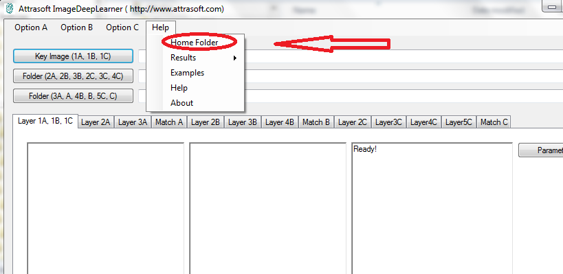
Figure 2.7 “.\” folder, the Home Folder.
The data folders are:
|
Layers |
Working
Folder |
Final
Folder |
|
2A |
.\layer2 |
. \data1 |
|
3A, A |
.\data |
.\data |
|
2B, 3B |
. \layer2b |
.\data1b |
|
4B, B |
.\data |
.\data |
|
2C, 3C, 4C |
. \layer2c |
. \layer1c |
|
5C, C |
.\data |
.\data |
The data files are:
|
Function |
Files
1 |
File
2 |
|
Training ( 3A, 4B, 5C) |
T1.txt |
Match.txt |
|
Retraining ( 3A, 4B, 5C) |
T2.txt |
Match2.txt |
|
Search library ( 3A, 4B, 5C) |
A1.txt |
|
|
Layer 2 features (2A, 2B, 2C) |
L*.txt |
|
|
Layer 3 features (3B, 3C) |
M*.txt |
|
|
Layer 4 features (4C) |
N.txt |
|
These files will overwrite themselves for each problem. To back up a
problem, you will need to manually save these files.
2.6 Again, What is Deep Learning
Mathematically, Deep Learning is a multi-layered transformation.
For example, assume we have several layers; let an input vector be:
A = ( a0, a1, …, a19).
Assume Layer-1 will have 4 segments:
B = (B0, B1, B2, B3)
= ( (b0, b1, b2, b3), (b4, b5, b6, b7), (b8, b9, b10, 11), (b12, b13, b14, b15) )
So the first layer has some simple transformations:
A è B0
Aè B1
Aè B2
Aè B3
Assume Layer-2 will have two segments:
C = (C0, C1)
= ( ( c0, c1, c2, c3), (c5, c6, c7, c8) )
So the second layer has some simple transformations:
(B0, B1) è C0
(B2, B3) è C1
Assume Layer-3 will have 1 segment:
D = (d0, d1, d2, d3)
So the third layer has a simple transformation:
(C0, C1) è D
The DeepLearner will operate this on a much larger scale.
2.7 Summary
To summarize, the DeepLearner has 4 distinct layers:
· Layers 1A, 1B, 1C identify line segments.
· Layers 2A, 2B, 2C create features from images or image segments.
· Layers 3B, 3C, 4C create features from features.
· Layers 3A, 4B, 5C identify the images.
3. Preparation Work for Three-Layer DeepLearner
In this chapter, we will list the preparation steps for the three-layer DeepLearner. Your work is mainly data organization. It is divided into three sections:
· Data for feature generation;
· Data for teaching the software what is a match;
· Data for testing the software;
· Data for saving software generated data.
3.1 Layer 1A: Line Detection
It is well established cross almost all literature that the first layer is to identify curves. Since there is much to be done, we will simply use the default setting. No preparation work is required for Layer 1A.
3.2 Layer 2A: Feature Engineering
Figure 3.1 Layer 2A of the DeepLearner.
Recall from Chapter 1: a representation of an image recognition problem is a table. For a given problem, there are many representations. A column of a representation table is called an Image Feature. A row of the table is called an Image Signature in this manual. The process to obtain a representation for images is called Feature Engineering.
In deep learning, feature engineering is an automatic process, meaning no programming is required.
Feature selections do have significant impact on the final computation results, so features must be collected carefully. There are two things you have to do in Layer-2A preparation.

Figure 3.2 An example of feature extraction data.
3.2.1 Feature Image Folder
The features are computed directly from the images; you will group similar images together and let the computer find common features among the images.
You will need to organize your problem in a master folder. There will be many folders inside; the first folder will be the feature folder.
Masterfolder
featureFolder
The first task you will do is to collect images. You classify images into several categories, so the feature folder will be further divided into many subfolders. Each subfolder will have images in the same category. Figure 3.2 offers an example; now the Master folder will look like this:
Masterfolder
featureFolder
feature1
feature2
feature3
…
3.2.2 Number of Features
The number of features you will get from each subfolder will be decided ahead of time. At the beginning, you should plan to obtain 500 to 1000 features. You will distribute this number among your subfolders of images.
For example, assume you want to get 20 features from folder, “feature1”; you want to get 25 features from folder, “feature2; … then rename your folders as follows:
Masterfolder
featureFolder
feature1_20
feature2_25
feature3_15
…
Now the feature folders are ready.
3.3 Layer 3A: Supervised Learning
Figure 3.3 Layer 3A of the DeepLearner.
It is well established cross almost all literature that the last layer is the learning layer. In this layer, you will teach the software what is a match.

Figure 3.4 Supervised learning folder.
Now your Master folder looks like this:
Masterfolder
featureFolder
learning
The DeepLearner allows you to define a match by image variation. You can also define your own match by image pairs. In either case, the matching definition process will generate many folders of images, such as rotation of a few degrees, so you will have many folders of data. We will discuss image variation generations later.
You can use the same data in feature engineering for training; however, you do need to reorganize the data.
In Layer 3A, the first time uses training; the rest of the time uses retraining. The training starts from the beginning by deleting old data. Retraining builds on top of existing training without deleting old data.
3.3.1 Training
Training teaches the DeepLearner what to look for. Training requires two files,
· t1.txt and
· match.txt
Both are generated automatically by the DeepLearner:
· T1.txt is the signature file, which contains a representation table. Each image is converted into a signature.
· Match.txt is a list of matching pairs. This file will teach the software who will match with whom.
3.3.2 Retraining
Retraining continues to teach the DeepLearner. Retraining can be repeated many times. Retraining requires two files, t2.txt and match2.txt. Now, the Master folder looks like this:
Masterfolder
featureFolder
feature1
feature2
feature3
…
learning
Training
Retraining1
Retraining2
….
3.4 Matching
Figure 3.5 Tab “Match A”.
At the end of the Layer 3A, the Deep Learning process is completed. Now, we move to the Matching-A tab to test. The Matching-A tab allows you to match one image against a folders of images.

Figure 3.6 Testing Folder.
Now, your Master folder looks like this:
Masterfolder
featureFolder
learning
testing
For testing, you will need a folder as an image library and a folder for testing images. A test image will match against a library. Now, the data folder looks like:
Masterfolder
featureFolder
feature1
feature2
feature3
…
learning
Training
Retraining1
Retraining2
….
Tesing
library
test
3.5 Graphical User Interface
The software is organized as:
· Option A
· Option B
· Option C
Option A is organized as:
· Layer 1
· Layer 2
· Layer 3
· Matching A
·
Redistributable A
Options B and C are similar. All examples can be accessed through the menu item, “Help/Example”.

Figure 3.7 Menu “Option A” will list all command to access the layers.

Figure 3.8 All the examples can be accessed through menu item, “Help/Examples”.
4. Three Layer Deep Learning
In this chapter, we will use a product/part identification example for the DeepLearner. Figure 3.8 opens this example.
4.1 Product Identification
The problem of product identification is this: given a product, what is its’ Product ID (Part ID, SKU, …)?
Figure 4.1 shows one example. Its application includes:
· Online order of a part;
· Replacing a damaged part;
· Placement of parts to correct locations;
· Delivering of parts to correct address;
· Value estimation of parts;
· …
|
|
Product |
Product ID |
|
1 |
|
0001 |
|
2 |
|
0002 |


Figure 4.1 Product Identification.
4.2 Dataset
Assume “.\” is the software home folder; this example is located in “.\examples\chap4” folder and can be accessed through menu item, “Help/Example” (Figure 3.8).
Figure 4.2 The dataset for feature extraction.
4.3 Layer 1A: Line Detection
Since there is much to be done, we will simply use the default setting.
4.4 Layer 2A: Automatic Feature Generation
Figure 4.3 Layer 2A of the DeepLearner.
Layer 2A builds features automatically from a folder of images. The process is given below (Figure 4.3):
1. Delete Old Data
2. Select a folder
3. Specify Number of Features.
4. Get Features
5. Check Results: get rid of almost black, almost white images.
6. Move the Feature data to its final location.
7. Repeat the above steps until all of the data folders are processed.
8. Final Results
Now we will walk through this process:
1. Click Button, “1. Delete Old Data (.\data1\*.*)
Click Button, “Delete
Old Data (.\data1\*.*), to delete the old problem. If you do not do this
step, the new problem will be added to the old problem.
2. Drag & drop a folder into the second text box (or click Button, “2. Select a folder”)
Drag & drop the first data folder into the second text box (or click Button, “2. Select a folder” to select a folder of images for extracting features).

Figure 4.4 Select a folder.
3. Enter 15 to the text box.
In the last chapter, Data Preparation, you have already prepared data for a project. You have also decided the number of features you will get from each subfolder. At the beginning, you should plan to obtain 500 or so features. You will distribute this number among your subfolders of images.
Assume we will get 15 features from the current folder; we will enter 15.

Figure 4.5 Specify Number of Features.
4. Click Button “4. Get Binary Features”
Click Button, “4. Get Binary Features”, to extract features from images.

Figure 4.6 Get Features.

Figure 4.7 Feature extraction for an image folder will take 1 second per image. When it is completed, a message will be printed: "Feature extraction completed!".
5. Click Button, “5. Check Results: get rid of bad images”
Click Button, “5. Check Results: get rid of bad images” to see the features visually. You will look through the features and delete images that are almost black, OR almost white, OR delete the images that are too close to others, OR something that you do not like.

Figure 4.8 Click Button, “5. Check Results: get rid of bad images”. In this case, all 15 features are acceptable.
6. Click Button, “6. Move Data (from .\layer2 to .\data1)
Click Button, “6. Move Data (from .\layer2 to .\data1), to move the computed features to its final location.
Click Button, “8. Final Results”; you will see these features have been moved to its final location in the Figure below.

Figure 4.9 Click Button, “8. Final Results”.
Before continuing, please note:
· In Deep Learning, features are generated completely automatically;
· In Deep Learning, features are generally data dependent. Data dependent features will ensure more accurate computations, at the cost of generality;
· In Deep Learning, features generally cannot be described by mathematical functions; i.e. the functions are directly defined by tables.
Your only involvements are:
· To prepare data;
· To specify the number of features from each subfolder.
7. Repeat the above steps until all of the data folders are processed.
Now, we have finished one folder of images. We will repeat the above 6 steps over and over again until all image folders are processed.
8. Final Results
See the final results for this layer which are visually represented by images, see Figure 4.9.
4.5 Layer 3A Data Organization
The third and last layer, Layer 3A, is the learning layer. In this layer, you will teach the software what is a match.
To teach the DeepLearner, you must prepare data. We assume that we will allow the following variations:
· Rotation of 2 degrees
· Rotation of - 2 degrees
· Scale 200%
In this example, we will limit it to these three variations.
Before we proceed, you need to organize your data in into three folders (See Figure below):
Train
Original
S200 (scale 200%)
Retrain1
Original
R002 (rotation 002 degree)
Retrain2
Original
R358 (rotation – 2 degree or 358 degree)

Figure 4.10 Organizing the data.
Each of these three folders will have two subfolders, the original images and the image variations. The original folder will contain the original images. After variation images have been generated, they will go to the other subfolders. In this example, the images here are the same images as the last section.
4.6 Layer 3A Data Generalization
In Figure 4.11, click Button, “0, Create Variations, match.txt”, to open a new form in Figure 4.12.
To generate variations, drag & drop the original image to the text box, see Figure 4.13. Now click one of the commands in Figure 14 to generate variations.
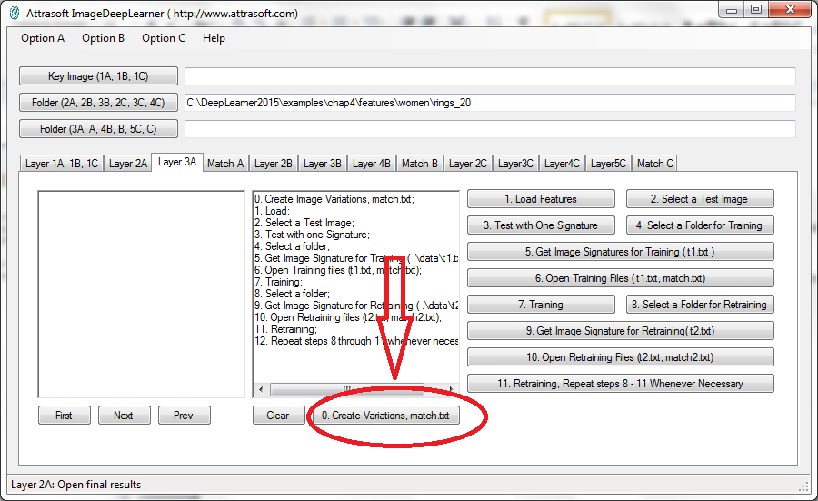
Figure 4.11 Click Button, “0, Create Variations, match.txt”, to create the training data.

Figure 4.12 Image Variation generation.

Figure 4.13 Drag & drop an image folder.

Figure 4.14(a) Scaling Commands. The commands scale the original images 150%, 200%, 300%, and 50%; or cut a few percent of the edges (5%, 10%, 15% or 20%).

Figure 4.14(b) Rotation Commands. The commands are rotation of 1, 2, 5, 10, -1, -2, -5, or -10 degrees.
Figure 4.14 Image Variation commands.
We assume that we will allow the following variations:
· Scale 200%
· Rotation of 2 degrees
· Rotation of negative 2 degrees
The corresponding commands are:
· Scaling/resize 200%
· Rotation/Rotate 2
· Rotation/Rotate -2
We will now generate the scale data:
· Drag & drop a folder
· Click a variation command
Allow some time for the variations to be generated; the computation will be finished when the images in Figure 4.15 stop changing.

Figure 4.15 Generating variations.
There are two results:
1. Click Button, “Open Folder”, in Figure 4.16 to see Figure 4.17; move these files to folders prepared in the last section:
Train
Original
S200 (scale 200%) ç
2. Click Button, “match.txt” in Figure 4.16 to see Figure 4.18; save this file to the “Train” folder above, see Figure 4.19.
We can repeat the above process two more times to complete generating all three variations:
o Scale 200%
o Rotation of 2 degrees
o Rotation of negative 2 degrees

Figure 4.16 Two results are generated.

Figure 4.17 Generated data.

Figure 4.18 Matching image information is contained in a text file.

Figure 4.19 Save match.txt.
4.7 Layer 3A: Supervised Learning
Layer 3A is a Supervised-Learning-Layer, which allows the software to learn what images will match with what other images. It is assumed that you have:
· completed Layer 2A, feature generation, and
· created Image Variations and match.txt
Layer 3A process is given below:
1. Load Features
2. Select a Test Image
3. Test with one Signature
4. Select a folder
5. Get Image Signature for Training ( .\data\t1.txt)
6. Open Training files (t1.txt, match.txt)
7. Training
8. Select a folder
9. Get Image Signature for Retraining ( .\data\t2.txt)
10. Open Retraining files (t2.txt, match2.txt)
11. Retraining
12. Repeat steps 8 through 11 whenever necessary.
Because we have three sets of data:
· Scale 200%
· Rotation of 2 degrees
· Rotation of -- 2 degrees
we will walk through the following process three times; each time with one of the following folders:
Train
Original
S200 (scale 200%)
Retrain1
Original
R002 (rotation 002 degree)
Retrain2
Original
R358 (rotation – 2 degree or 358 degree)
Each folder has about 7,000 images; and three folders have 21,000 images. It will take about 1 second per image; so this step will take a whole day to complete. We now start:
1. Click Button, “1. Load Features”
Click Button, “1. Load Features”, to load the Feature data from the last layer.
2. Click Button, “2. Select a Test Image”
Before starting with thousands of images, we will test the layer with one image first. Click Button, “2. Select a Test Image”, to select a test image. Go to Tab 1A, a single image will appear in Tab 1A.

Figure 4.20 Selecting an image.
3. Click Button, “3. Test with one Signature”
Go back to Tab 3A and test with one image signature computation. Click Button, “3. Test with one Signature”, and wait for OK message.
4. Drag & drop the first data folder into the third text box or Click Button, “4. Select a folder”
Dragging & dropping the first data folder into the third text box will select a folder for obtaining image signatures.

Figure 4.21 Selecting a folder.
5. Click Button, “5. Get Image Signature for Training ( .\data\t1.txt)”
Click Button, “5. Get Image Signature for Training ( .\data\t1.txt)”, to compute image signatures. The speed of this is 1 image/second, so this step will take a while until the DeepLearner prints:
Save to file: C:\DeepLearner2015\data\t1.txt
Please refer to Chapter 1 for the definition of Representation, features, image signatures, and feature engineering.
6. Click Button, “6. Open Training files (t1.txt, match.txt)”
Click Button, “6. Open Training files (t1.txt, match.txt)” to open these two files for training, t1.txt and match.txt:
·
T1.txt is
the signature file computed in the last step, which contains many signatures.
Each image is converted into a signature. Now you can close this file. Save
this file to the “Train” folder to make a backup copy.
·
Match.txt is
a list of matching pairs. This file will teach the layer who will match with
whom. You have created a file in Figure 4.18 and saved it to a location in
Figure 4.19; now you will:
o Open the saved match.txt;
o Copy and paste the content to the current
match.txt;
o Save.
To summarize:
·
Copy “.\data\t1.txt” to “.\examples\chap4\learning\train\t1.txt”;
·
Copy “.\examples\chap4\learning\train\match.txt”
to “.\data\match.txt”.
7. Click Button, “7. Training”
Click Button, “7. Training”, to train this layer. Wait for a message: “Neural Filter Training Completed!”. This will complete the processing of the first of the three folders:
o Train
o Retrain1
o Retrain2
Processing the next two folders will be very similar with an exception of clicking the retrain button.
8. Drag & drop the second data folder, “.\examples\chap4\learning\retrain1”, into the third text box or Click Button, “8. Select a folder”.
Now, we will repeat the above steps. This step selects the second data folder, “.\examples\chap4\learning\retrain1”, to obtain image signatures.
9. Click Button, “9. Get Image Signature for Retraining ( .\data\t2.txt)”
Click Button, “9. Get Image Signature for Retraining ( .\data\t2.txt)”, to compute image signatures for retraining. The first time uses training; the rest of the time uses retraining. The training starts from the beginning and the retraining builds on top of existing training.
10. Click Button, “10. Open Retraining files (t2.txt, match2.txt)”
Retraining requires two files, t2.txt and match2.txt; Click Button,
“10. Open Retraining files (t2.txt, match2.txt)”, to open
these two files. This step will:
·
Copy “.\data\t2.txt”
to “ .\examples\chap4\learning\train\t2.txt”;
·
Copy “.\examples\chap4\learning\retrain1\match2.txt” to “.\data\match2.txt”.
11. Click Button, “11. Retraining”
Click Button, “11. Retraining”, to retrain
this layer. Wait for a message: “Neural Filter Training Completed!”.
12. Repeat steps 8 through 11 one more time for the third folder.
This completes Layer 3A; now you have constructed the DeepLearner with three-layers. There are two more steps:
· Testing
· Creating redistribution software
These two topics will be introduced in the next chapter.
5. Redistribution Software
The DeepLearner is a software production tool without programing. In this chapter, we will:
· Test
· Create redistribution software
5.1 1:N Whole Matching Testing
Figure 5.1 Tab “Match A”.
When the DeepLearner is trained, it will be able to identify images. The initial testing is done on Tab A. Once the testing is done, a separate software is created with the image matching buttons only.
The testing process is:
1. Load Features
2. Select an image folder for searching
3. Get Image Signature ( .\data\a1.txt)
4. Load image library ( .\data\a1.txt)
5. Select a test Image
6. Whole image 1:N search
7. Image segment 1:N search
8. N:N search for evaluation
9. Check results for accuracy (b1.txt vs b1_matchlist.txt)

Figure 5.2 Test Data.
The test folder is the “chap4\tesing\library” folder below:
Masterfolder
featureFolder
learning
train
retrain1
retrain2
testing
Library
test
The testing data is exactly the same as “chap4\learning\retrain2”.
The details are:
1. Click Button, “1. Load Features”
Click Button, “1. Load Features”, to load the Feature data from the last layer. When step is completed, a message, “Feature loaded!, …” will be printed.
2. Drag & drop a folder to the third text box or Click Button “2. Select an Image Folder for Searching”
Drag & drop a folder to the third text box:
. \examples\chap4\testing
Note that the
picture box in this tab and text window are for showing results; so you will
not see the selected images in this tab; instead, the selected images are displayed in Tab 3A.
3. Click Button, “3. Get Image Signature ( .\data\a1.txt)”
Click Button, “3. Get Image Signature ( .\data\a1.txt)”, to compute image signatures. This step will take a while.
4. Click Button, “4. Load image library ( .\data\a1.txt)”
Click Button, “4. Load image library ( .\data\a1.txt)”, to load image signatures from file, .\data\a1.txt. When is step is completed, a message, “Library List loaded!”, will be printed.
5. Drag & drop an image to the first text box or Click button, “5. Select a test Image”
Dragging & dropping an image to the first text box selects an image for testing. Note that the picture box and text window are for showing results; so you will not see the selected image in this tab; instead, the selected image is displayed in Tab 1A.

Figure 5.3 Dragging & dropping an image to the first text box selects an image for testing.
6. Click Button, “6. Whole image 1:N search”
Click Button, “6. Whole image 1:N search”, to match the selected image against the selected folder. The results look like the following two figures.

Figure 5.4 1:N matching text output.

Figure 5.5 Matched images. Click the next button to get the next matched image.
5.2 1:N Partial Image Identification
Now we go inside an image and match a portion of the image with the library.
7. Click Button, “7. Image segment 1:N search”
Click Button, “7. Image segment 1:N search”, to match partial images segments from the selected image against the selected folder. This button will go inside image and match a portion of the selected image to the library.

Figure 5.6 Matched image segments. Click the next button to get the next matched image segments.
5.3 Multiple Search
Now we will make an N:N match. There are N = 7,288 images, so each of the N images will be matched against N images, which will make 53 million matches, so this step will take a while.
8. Click Button, “8. N:N search (a1.txt vs Lib)”
Click Button, “8. N:N search (a1.txt vs Lib)”, to match every image in the selected folder against the same folder. When completed, a text file will be opened, which lists all of the matching pairs. There are 139,860 matches. 139,860 is about 0.26% of the 53 million possible matches. The results are saved in “.\data\b1.txt”.

Figure 5.7 N:N matching text output. The results are saved in “.\data\b1.txt”.
5.4 Evaluation of the Software
Since these images are from the training2 folder, we know which images should match with which images; they are image pairs from file, “.\data\match.txt”. Open and save this file to “.\data\b1_matchlist.txt”. The results of N:N matching are stored in “.\data\b1.txt”. The last button will compare these two lists.
9. Click Button, “9. Check results for accuracy (b1.txt vs b1_matchlist.txt)”
Click Button, “9. Check results for accuracy (b1.txt vs b1_matchlist.txt)”, to analyze the results of an N:N match. B1.txt contains computer generated N:N matching results. B1_matchlist contains the matching image pairs. This button will report the percentages of the image pairs found in both files. In this case, it reports 3641 matches. The total number of matches is 3644. The three missing matches represent a match score that is lower than the threshold.
5.5 Generating Redistribution Software
To generate the redistribution software, click “Create Software” button. A message, “Software created!” will be printed when finished. After that, click button “Open Software” to open the software folder. All files in this folder will be required to redistribute.

Figure 5.8 Generate redistribution software.

Figure 5.9 Open the redistribution software folder.
5.6 How to Use Redistribution Software
Click the CustomizedImageFinder.exe file to run, see figure below:

Figure 5.10 Run the redistribution software.
The testing process is:
0. Initialization (Load Features and existing image library)
1. Select an image folder for searching
2. Get Image Signature ( .\data\a1.txt)
3. Select a test Image
4. Whole image 1:N search
5. Image segment 1:N search
As we created the software, the last image signature library will also be copied. The button, “0. Initialization (Load Features and existing image library)”, will load both the features and the existing library; so after clicking this button, the software is ready to search. Now drag and drop an image to the second text box and click “4. Whole Search” to make an 1:N search, see Figures below.

Figure 5.11 1:N matching in the redistribution software.

Figure 5.12 Results from 1:N matching in the redistribution software.
6. Four-Layer Architecture
There are many reasons to go beyond the minimum architecture. One reason is image tagging and concept identification. Another reason is that an object can have a hierarchy. For example, the objects to be identified have multiple parts organized into a hierarchy:
Figure 6.1 A pair of earrings with different separation distance.
The 4-layer architecture is called Option B. Option B has 4 layers:
· Layer 1B identifies lines.
· Layer 2B creates features from the four quarters of each image.
· Layer 3B creates new features from the four features in Layer 2B.
· Layer 4B identifies the images.
6.1 Concept Identification
We will explain the difference between product identification and concept identification:
Figure 6.2a identifies the product as a particular ID. Two different watches will have two different ID.
Figure 6.2b identifies the product as watch. Two different watches will have the same tag.
|
|
Product |
Product ID |
|
1 |
|
0001 |
|
2 |
|
0002 |
(a) Product Identification.
|
|
Product |
Product ID |
|
1 |
|
Watch |
|
2 |
|
Ring |
(b) Concept Identification.
Figure 6.2 Difference between product identification and concept identification.
The reasons to use the deep learning architecture for concept identification is this:
as we move from a lower layer to a higher layer, some fine details are blurred; i.e. the higher layer is less sensitive to fine details than the lower layers. As a result, objects from basically the same category are grouped together in the higher layers.
6.2 Layer 1B
This layer identifies lines and curves. We suggest you use the default setting and ignore the entire layer.
6.3 Layer 2B

Figure 6.3 Layer 2B.
This layer builds features automatically from a folder of images. The data for this chapter is stored in:
.\examples\chap6\
This example will identify three concepts:
· Earrings
· Rings
· Watches
The numbers of features are:
· Earrings, 500 per segment, 2000 total
· Rings, 500 per segment, 2000 total
· Watches, 100 per segment, 400 total
The organization of the data is similar to the earlier example. All the examples can be accessed through menu item, “Help/Examples”.

Figure 6.4 Chapter 6 Example.
The process is given below:
1. Delete Old Data
Click “1. …” button.
2. Select a folder
Drag & drop the following folder to the second text box:
.\examples\chap6\features\earrings_500
3. Specify Number of Features
The numbers of features to be entered are (Figure 6.5):
· Earrings, 500
· Rings, 500
· Watches, 100
4. Get Features
Click “4. …” button. Figure 6.5 shows the DeepLearner running. This step will take a long time.

Figure 6.5 Click “4. …” button.
5. Check Results
Click “5. …” button.

Figure 6.6 Click “5. …” button.
6. Move the Feature data to its final location.
Click “6. …” button.
7. Repeat the above steps until all of the data folders are processed.
8. Final Results
Click “8. …” button.

Figure 6.7 Click “8. … “ button.
Note:
Step 6 can be done only once for each folder of images; otherwise, it will add to the existing features multiple times.
This example
will take a whole day to run.
This layer generated 4400 features; the next layer will reduce the number of features to 440.
6.4 Layer 3B

Figure 6.8 Layer 3B.
Layer 3B builds features automatically from four features obtained in Layer 2B. The process of Layer 3B is identical externally to Layer 2B. Internally,
· Layer 2B obtains features directly from each of the four quarters of each image.
· Layer 3B obtains features from four features from Layer 2B.
The process is given below:
1. Delete Old Data
2. Select a folder
3. Specify the Number of Features:
We will run three folders:
· Earrings, 200
· Rings, 200
· Watches, 40
4. Get Features
5. Check Results
6. Move the Feature data to its final location
7. Repeat the above steps until all of the data folders are processed
8. Final Results
We have repeated this process several times by now, so we will omit the details.
6.5 Layer 4B Data Generalization

Figure 6.9 Layer 4B.
We have gone through the process of generating variations before. The data for this section is located in:
.\examples\chap6\learning\train\original\

Figure 6.10 The data.
We assume that we will allow the following variations:
· Scale 200%
· Rotation of 2 degrees
· Rotation of negative 2 degrees
In Figure 6.9, click Button, “0, Create Variations, match.txt”, to open a new form in Figure 6.11.
To generate variations, drag & drop the original image folder,
.\examples\chap6\learning\train\original\
to the text box, see Figure 6.12.
Figure 6.11 Image Variation generation.

Figure 6.12 Drag & drop an image folder.
Click the following menu items to generate the variation (See Figure 6.13):
· Scaling/Resize 200%
· Rotation/Rotate 2
· Rotation/Rotate -2

Figure 6.13 Generating variations.
There are two results, image variations and a file of matching pairs:
1. Click Button, “Open Folder”, and move these files to folder:
.\examples\chap6\learning\train\S200\
2. Click Button, “match.txt”; save this file to folder:
.\examples\chap6\learning\train\
We can repeat the above process two more times to complete generating all three variations:
o Scale 200%
o Rotation of 2 degrees
o Rotation of negative 2 degrees

Figure 6.14 Copy & paste the file, match.txt.
6.6 Training
The last layer is a Supervised-Learning-Layer, which allows the software to learn what images will match with what other images. It is assumed that you have completed Layers 2B and 3B before you move to this layer. The process is identical to Layer 3A introduced earlier:
1. Load Features
2. Select a Test Image
3. Test with one Signature
4. Select a folder
5. Get Image Signature for Training ( .\data\t1.txt)
6. Open Training files (t1.txt, match.txt)
7. Training
8. Select a folder
9. Get Image Signature for Retraining ( .\data\t2.txt)
10. Open Retraining files (t2.txt, match2.txt)
11. Retraining
12. Repeat steps 8 through 11 whenever necessary.
Details:
1. Load Features
Click “1. …” button.
2. Select a Test Image
Drag & drop an image to the first text box.
3. Test with one Signature
Click “3. …” button and wait for message “Test OK!”.
4. Select a folder
Drag & drop the following folder to the third text box:
.\examples\chap6\learning\train\
5. Get Image Signature for Training ( .\data\t1.txt)
Click “5. …” button and wait for message:
Save to file : C:\DeepLearner2015\data\t1.txt
6. Open Training files (t1.txt, match.txt)
Click “6. …” button to open two training files, t1.txt, match.txt, copy the contents from file,
.\examples\chap6\learning\train\match.txt
to
.\data\match.txt

Figure 6.15 Copy & paste from file, “.\examples\chap6\learning\train\match.txt” to “.\data\match.txt”.
7. Training
Click “7. …” button and wait for message:
Training Completed!
Now let us save this file; open file:
.\data\t1.txt
Save it to
.\examples\chap6\learning\train\t1.txt
8. Select a folder
Now we continue retraining. Drag & drop the following folder to the third text box:
.\examples\chap6\learning\retrain1\
9. Get Image Signature for Retraining ( .\data\t2.txt)
Click “9. …” button and wait for message:
Save to file : C:\DeepLearner2015\data\t2.txt
10. Open Retraining files (t2.txt, match2.txt)
Click “10. …” button to open two retraining files, t2.txt, match2.txt, copy the contents from file,
.\examples\chap6\learning\retrain1\match.txt
to
.\data\match2.txt
11. Retraining
Click “11. …” button and wait for message:
Retraining Completed!
Now let us save this file, open file:
.\data\t2.txt
Save it to
.\examples\chap6\learning\retrain1\t2.txt
12. Repeat steps 8 through 11 for the folder:
.\examples\chap6\learning\retrain2\.
6.7 Testing

Figure 6.16 Testing with Tab “Match B”.
When the DeepLearner is trained, it will be able to identify images. The initial testing is done on Tabs A, B, and C, respectively. Once the testing is done, a separate software is created with the image matching buttons only.
The testing process is:
1. Load Features
2. Select an image folder for searching
3. Get Image Signature ( .\data\a1.txt)
4. Load image library ( .\data\a1.txt)
5. Select a test Image
6. Whole image 1:N search
7. Image segment 1:N search
8. N:N search for evaluation
9. Check results for accuracy (b1.txt vs b1_matchlist.txt)
Details:
1. Load Features
Click “1. …” button.
2. Select an image folder for searching
Drag & drop the following folder to the third text box:
.\examples\chap6\learning\train\original\
3. Get Image Signature ( .\data\a1.txt)
We have obtained the signature in the last section; now we simply save it to a different file.
Open file:
.\examples\chap6\learning\train\a1.txt
Save it to
.\data\a1.txt
4. Load image library ( .\data\a1.txt)
Click “4. …” button and wait for message:
Library List loaded!
5. Select a test Image
Drag & drop an image to the first text box from folder:
.\examples\chap6\testing\test\
6. Whole image 1:N search
Click “6. …” button until you see the results.
The purpose here is to identify three types:
· Earrings
· Rings
· Watches
Select a ring: we will get majority of matching images being rings, which indicate the ring being the matching type.
6.8 Image Segment Search
To match a segment of the selected image with the library, click button, “7. Image segment 1:N search”. This process is identical to Section 5.2 except it is in Tab B.
6.9 N:N Match
To make an N:N match, click button, “8. N:N Match”. This process is identical to Section 5.3 except it is in Tab B.
6.10 Evaluations
To evaluate the results of an N:N match, click button, “9. Check results for accuracy (b1.txt vs b1_matchlist.txt)”. This process is identical to Section 5.4 except it is in Tab B.
6.11 Generating Redistributable Software
To generate the redistribution software, click “Create Software” button. A message, “Software created!” will be printed when finished. After that, click button “Open Software” to open the software folder. All files in this folder will be required to redistribute. This process is identical to Section 5.5 except it is in Tab B.
7. Five-Layer Architecture
When many layers are used, in general, it is for concept recognition. The 5-layer architecture is called Option C. Option C has 5 layers:
· Layer 1C identifies lines.
· Layer 2C creates features from nine image segments from each image.
· Layer 3C creates four new features, each from four features in Layer 2C.
· Layer 4C creates one new feature from four features in Layer 3C.
· Layer 5C identifies the images.
We will use an example to show the process, which will identify several concepts. The example is located at:
.\examples\chap7\
7.1 Layer 1C
This layer identifies lines and curves. We suggest you use the default setting and ignore the entire layer.
7.2 Layer 2C

Figure 7.1 Layer 2C.
This layer builds features automatically from a folder of images. The data for this chapter is stored in:
.\examples\chap7\
This example will identify several random concepts:
· Beach
· Car
· Ships
· House
· TV
The numbers of features are specified in the Figure below. The organization of the data is similar to the earlier example. All the examples can be accessed through menu item, “Help/Examples”.

Figure 7.2 Chapter 7 Example.
The process is given below:
1. Delete Old Data
Click “1. …” button.
2. Select a folder
Drag & drop the following folder to the second text box:
.\examples\chap7\features\beach_200
3. Specify the Number of Features
Enter the number of features to the text box:
o Beach, 200
o Car, 200
o Ships, 200
o House, 400
o TV, 200
4. Get Features
Click “4. …” button. This step will take a long time.
5. Check Results
Click “5. …” button.
Reduce the number of features from each folder to 200.

Figure 7.3 Click “5. …” button.
6. Move the Feature data to its final location
Click “6. …” button.
7. Repeat the above steps until all of the data folders are processed.
8. Final Results
Click “8. …” button.

Figure 7.4 Click “8. …” button.
Note:
Step 6 can be done only once for each folder of images; otherwise, it will add to the existing features multiple times.
This example
will take several days to run.
7.3 Layer 3C

Figure 7.5 Layer 3C.
Layer 3C builds features automatically from four features obtained in Layer 2C. The process of Layer 3C is identical externally to Layer 2C. Internally,
· Layer 2C obtains features directly from each of the four quarters of each image.
· Layer 3C obtains features from four features from Layer 2C.
The process is given below:
1. Delete Old Data
2. Select a folder
3. Specify Number of Features:
We will run five folders:
o Beach, 200
o Car, 200
o Ships, 200
o House, 400
o TV, 200
4. Get Features
5. Check Results
6. Move the Feature data to its final location
7. Repeat the above steps until all of the data folders are processed
8. Final Results
We have repeated this process several times by now, so we will omit the details.
7.4 Layer 4C

Figure 7.6 Layer 4C.
Layer 4C builds features automatically from four features obtained in Layer 3C. The process of Layer 4C is identical externally to Layer 3C. The process is given below:
1. Delete Old Data
2. Select a folder
3. Specify the Number of Features
We will run five folders:
o Beach, 200
o Car, 200
o Ships, 200
o House, 400
o TV, 200
4. Get Features
5. Check Results
6. Move the Feature data to its final location
7. Repeat the above steps until all of the data folders are processed
8. Final Results
We have repeated this process several times by now, so we will omit the details.
7.5 Layer 5C Data Generalization

Figure 7.7 Layer 4C.
We have gone through the process of generating variations twice in section 4.6 and 6.5. The data for this section is located in:
.\examples\chap7\learning\train\original\

Figure 7.8 The data.
We assume that we will allow the following variations:
· Rotation of 2 degrees
In Figure 7.7, click Button, “0, Create Variations, match.txt”, to open a new form in Figure 7.9. To generate variations, drag & drop the original image folder,
.\examples\chap7\learning\train\original\
Please see sections 4.6 and 6.5.
Figure 7.9 Image Variation generation.
7.6 Training
The last layer is a Supervised-Learning-Layer, which allows the software to learn what images will match with what other images. It is assumed that you have completed Layers 2C, 3C, and 4B before you move to this layer. The process is identical to Layer 3A and 4B introduced earlier:
1. Load Features
2. Select a Test Image
3. Test with one Signature
4. Select a folder
5. Get Image Signature for Training ( .\data\t1.txt)
6. Open Training files (t1.txt, match.txt)
7. Training
8. Select a folder
9. Get Image Signature for Retraining ( .\data\t2.txt)
10. Open Retraining files (t2.txt, match2.txt)
11. Retraining
12. Repeat steps 8 through 11 whenever necessary.
Details:
1. Load Features
Click “1. …” button.
2. Select a Test Image
Drag & drop an image to the first text box.
3. Test with one Signature
Click “3. …” button and wait for message “Test OK!”.
4. Select a folder
Drag & drop the following folder to the third text box:
.\examples\chap7\learning\train\
5. Get Image Signature for Training ( .\data\t1.txt)
Click “5. …” button and wait for message:
Save to file : C:\DeepLearner2015\data\t1.txt
6. Open Training files (t1.txt, match.txt)
Click “6. …” button to open two training files, t1.txt, match.txt; copy the contents from file,
.\examples\chap7\learning\train\match.txt
to
.\data\match.txt

Figure 7.10 Copy & paste from file, “.\examples\chap6\learning\train\match.txt” to “.\data\match.txt”.
7. Training
Click “7. …” button and wait for message:
Training Completed!
Now let us save this file; open file:
.\data\t1.txt
Save it to
.\examples\chap6\learning\train\t1.txt
7.7 Testing

Figure 7.11 Testing with Tab “Match C”.
When the DeepLearner is trained, it will be able to identify images. The initial testing is done on Tabs A, B, and C, respectively. Once the testing is done, a separate software is created with the image matching buttons only.
The testing process is:
1. Load Features
2. Select an image folder for searching
3. Get Image Signature ( .\data\a1.txt)
4. Load image library ( .\data\a1.txt)
5. Select a test Image
6. Whole image 1:N search
7. Image segment 1:N search
8. N:N search for evaluation
9. Check results for accuracy (b1.txt vs b1_matchlist.txt)
Details:
1. Load Features
Click “1. …” button.
2. Select an image folder for searching
Drag & drop the following folder to the third text box:
.\examples\chap7\learning\train\original\
3. Get Image Signature ( .\data\a1.txt)
Drag & drop the following to the third text box:
C:\DeepLearner2015\examples\chap7\learning\train\original
Click button, “3. Get Image Signature ( .\data\a1.txt)”.
4. Load image library ( .\data\a1.txt)
Click “4. …” button and wait for message:
Library List loaded!
5. Select a test Image
Drag & drop the first image to the first text box from folder:
.\examples\chap7\testing\test\
We will continue in the next section.
7.8 Parameters

Figure 7.12 Parameter button.

Figure 7.13 Parameter Window.

Figure 7.14 Setting Parameters for Layers 3A, A, 4B, B, 5C and C.
This problem requires setting the parameter. Go to Tab 1A in Figure 7.12 and click the “Parameter” button, you will see Figure 7.13. In Figure 7.13, click button ‘NF Parameters’ and you will see Figure 14. Set:
Fault Tolerance Scale 0
Blurring 0
Sensitivity 0
Threshold 99
Now we go back to Tab C and continue the example from the last section.
6. Whole image 1:N search
Click “6. …” button until you see the results.
The results will have some mixing results; consider each match is one point. The classification that has the most points is the computed classification. The house image will have the most matches in house images, indicating the tagged word is house.
7.9 Image Segment Search
To match a segment of the selected image with the library, click button, “7. Image segment 1:N search”. This process is identical to section 5.2 except it is in Tab C.
7.10 N:N Match
To make an N:N match, click button, “8. N:N Match”. This process is identical to section 5.3 except it is in Tab C.
7.11 Evaluations
To evaluate the results of an N:N match, click button, “9. Check results for accuracy (b1.txt vs b1_matchlist.txt)”. This process is identical to section 5.4 except it is in Tab C.
7.12 Generating Redistributable Software
To generate the redistribution software, click “Create Software” button. A message, “Software created!” will be printed when finished. After that, click button “Open Software” to open the software folder. All files in this folder will be required to redistribute. This process is identical to Section 5.5 except it is in Tab C.
8. Related Issues
8.1 Video User’s Guide
The video user’s guide can be found on YouTube. The addresses are:
8.2 Potential Uses
We have listed some potential applications below:
(a) Employees cannot memorize large amounts of images (in the order of 1000); manual image identification in such cases take a long time.
(b) Employees cannot memorize large amounts of images (in the order of 1000); manual image identification in such cases will have many errors.
(c) Automated image search to locate engineering drawings, graphs, charts, architectural designs, maps, document images, logos, etc. are required in many applications.
(d) Assigning keywords to images can be labor intensive and expensive.
(e) Some images, when described by keywords, will yield millions of results, producing low relevancy.
(f) Some images cannot be accurately described by keywords.
(g) Some images can be difficult to describe via keywords; for example, there are 70,000 car wheel rims styles, and “car wheel rim” can mean one of 70,000 different objects.
(h) Some images can be mislabeled (human error or intentional).
(i) Government / Law Firms need an automated search to identify Patent drawings / trademarks and more.
(j) Keyword search does not group a specific image well in search results (similar images are separated by many images).
(k) For many applications both image index search and image direct search are required.
(l) Etc., …
8.3 Customized Software and Services
Attrasoft will also customize the software for:
· Scale
· Rotation
· Translation
· Flipping
· Lighting Conditions
· Different Data Acquisition Devices (camera vs. scanner)
· Catalog images vs. Operation images
· Searching for an object in an image
· Different Interface
· Licensing the technology
· …
In addition, if you need services, such as:
· Attrasoft will train the ImageDeepLearner for you with your data
· Attrasoft can design Deep Learning Architecture for you for your application
· Mini-AttraSeek Hosting Service
· Monitoring specific websites for illegal use of brand specific images
· Video Search: Download Demo (http://attrasoft.com)
· Video Index
· ID Image Duplication Verification
· Trademark Identification
· …
8.4 Types of License, Software Limits, and Support
ImageDeepLearner has three different types of license:
· Personal License;
· Business License;
· Commercial License.
This package is for the personal use only, which has the following limitations:
·
You cannot sell a service based any computation
results produced by this software.
o
You must
purchase a separate annual license for commercial use from Attrasoft.
·
You cannot use the software to perform work for
which you will get paid for.
o
You must
purchase a separate annual license for business use from Attrasoft.
·
You cannot build software on top of this
software.
o
You must
purchase a separate annual license for redistribution from Attrasoft.
The ImageDeepLearner will search up to 10,000 images in a folder, including all images in subfolders. The 10,000 limit is generous for personal use.
Beyond this limit, a customized version can be ordered from Attrasoft. These versions require an annual license subscription instead of one-time fee:
· 50,000 version (2x annual license);
· 100,000 version (3x annual license);
· 200,000 version (4x annual license);
· 400,000 version (5x annual license);
· 800,000 version (6x annual license);
· 1,600,000 version (7x annual license);
· …
For a Business Annual Subscription, Commercial Annual Subscription, or a Redisturibution Annual Subscription, please contact Attrasoft at gina@attrasoft.com.
8.5 Q & A
Q: What are ImageDeepLearner’s
running requirements?
A: Microsoft Windows.
Q: What are scores?
· Absolute match: 99% - 100%
· Good matches: 90% - 98%
· Somewhat matches: 83% - 89%
· Possible Similarities: 80% - 82%
· Few Similarities: <80%.
Q: Can you search Video?
A: The difference between video search and image search is that a video has a lot more images. Attrasoft VideoFinder deals with videos.
Q: How to handle multiple image searches?
A: Yes, the ImageDeepLearner can handle multiple image searches; please refer to sections related to multiple searches.
Q: Can I rotate a Test Image and then
search?
A: Two options: (1) rotate the images and add it to the library; or (2) order a customized version.
Q: Can I clip a portion out of a Test Image
and then search?
A: The current version searches 30 sub-images inside an image. More searching can be handled in a customized version.
Q: What is Customized software?
A. Customized software can be built for special requirements such as:
· Variation of images such as scale, rotation, flipping, lighting condition(s),
· Different data acquisition devices (camera vs. scanner),
· Catalog images vs. operation images, etc,
· Searching for an object in an image,
· A different web interface,
· A document image search,
· Fine-tuning internal parameters or programming,
· Emphasizing speed, i.e. it can search a huge amount of images very fast,
· Licensing the technology.
Q: Can I contract Attrasoft to train the DeepLearner for my application?
A. Yes. Contact gina@attrasoft.com if you would like to contract
Attrasoft to train the DeepLearner for your application (skip pre-training the
DeepLearner and go directly to using the software for your application).
Contact: gina@attrasoft.com