3.1 Step 1: Training and Testing Format
Chapter 2 is the quick version of the manual, which listed the minimum requirements. After chapter 2, you should be able to operate the software. However, a few details were left out in chapter 2, such as, what is symmetry and how to set up symmetry.
Chapter 3 and 4 will present a detailed user's guide. There will be some repetition between chapter 2 and chapter 3.
The operation has 4 steps:
Step 1. Put your training data into a file, the training file; Put your problem or test data into another file, the testing file; together you prepare two files.
Step 2. Link the two files to the ABM by clicking "Data/Link".
Step 3. Once the files are in the ABM, set up symmetry and output format for ABM if necessary;
Step 4. Click "Run/Classification" or "Run/Distribution".
The command, "Run/Distribution", presents you with a distribution, which is all possible classifications and how valuable the ABM thinks each prediction is via a confidence number. This number is similar to the number in an Internet Search Engine: the higher that number, the more confidence the ABM has in that distribution.
The command, "Run/Classification", presents you with a classification, and a confidence number; the higher this number, the more confidence the ABM has in that classification.
3.1 Step 1: Training and Testing Format
The best way to learn the two file formats is to look at the examples in the ABM, for example, click "Example/Character5x7". The format is very easy to learn.
An example of a training file is:
5x7 Character Recognition: Training File
Add your data at the end
*
46
10000000000
01000
10100
10100
01000
00000
00000
00000
10000000000
01000
10100
10100
10100
01000
00000
00000
5x7 Character Recognition : Testing File
*
xxxxxxxxxxx
00100
01010
01010
01010
01010
00100
00000
Training Files Testing Files
----------------------------- ----------------------
Comment Section
Comment Section
Neuron Number Section
Data Section
Data Section
The two files must be prepared in the text file format. The ABM has its own text editor. Or if you wish, you can use any word processor, like Microsoft Word, or WordPerfect; just make sure you save the data file in the text format.
The training file has three sections:
Part 1 of the Training
File: Comment Section
The comment section starts with a "*" and ends with another "*". The purpose of this section is to document your data:
Title: 5 x7 character recognition
Data: 0, 1, ..., 9
*
Part 2 of the Training File: Number of Neurons
This section has a single integer, which will tell the ABM how many neurons you will use.
In the 5x7 character recognition example, each 5x7 character
takes 35 neurons, and the number of classes is 11, giving a total of 35
+ 11 = 46 neurons.
Part 3 of the Training File: Data Section
This section contains the data.
Example
Character Recognition: Training File
Add your data at the end
*
46
10000000000
01000
10100
10100
01000
00000
00000
00000
10000000000
01000
10100
10100
10100
01000
00000
00000
10000000000
01000
10100
10100
10100
10100
01000
00000
10000000000
01000
10100
10100
10100
10100
10100
01000
10000000000
01100
10010
10010
01100
00000
00000
00000
...
This section is the same as the comment section of the
training file.
Part 2 of the Test File: Data Section
This section is the same as the data section of the training file, however, each pattern contains unknown bits, xxx...xxx. ABM will convert the unknown bits to a string of 0's and 1's.
The rules for the testing files are:
(1) The unknown bits in a testing file must be marked as 'x';
(2) The unknown bits in a testing file must stay together;
(3) The unknown bits in a testing file must be the same position.
The following test pattern is wrong because x's are
separated:
100 xx11 xx10,
The following test pattern is wrong because y's are
illegal characters:
100 yyyy 0110,
The following test pattern is wrong because x's are
not in the same position:
100 xxxx 0110,
100 00xx xx10.
If you want ABM to fix:
100 xxxx 0110,
100 00xx xx10,
you have to run twice, the first time with the testing
pattern
100 xxxx 0110,
and the second time with the pattern
100 00xx xx10.
Example
xxxxxxxxxxx
00100
01010
01010
01010
01010
00100
00100
xxxxxxxxxxx
00000
00100
01010
01010
01010
01010
00100
3.2 Step 2: Link Input Files To ABM
There are two input files to be linked:
Method 1:
C:\Program Files\Attrasoft\ABM 2.7\Example1a.txt
C:\Program Files\Attrasoft\ABM 2.7\Example1b.txt
If you are using two files for a problem over and over again, you can use the following method to link:
Method 3:
C:\Program Files\Attrasoft\ABM 2.7\Example1b.txt
Let a string be 101, then the position of the first bit
is 0; the position of the second bit is 1; and the position of the third
bit is 2, ...
position: 012,
pattern: 101.
Similarly, the position of another pattern 1010 1100
is:
position: 0123 4567,
pattern: 1011 1100.
If no output format is given, the default will print one pattern per line.
If your testing pattern is long, or they are 2-dimensional, you might want to change this default format. Inserting line breakers will do just that.
ABM allows you to insert up to 4 line breakers.
To insert the line breakers, you must specify the positions of the line
breakers. Suppose you want the output look like this:
111
0000
11111
000000
1111111
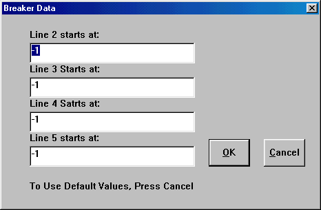
then click: "Data/Line Breaker" and specify (See Figure
6):
Line 2 starts at 3
Line 3 starts at 7
Line 4 starts at 12
Line 5 starts at 18.

Figure 6. Set up Line Breakers.
The position of the first bit is 0; the position of the second bit is 1; and the position of the third bit is 2. Note that after "111", the next position is 3. "Line 2 starts at 3" means a new line starts after "111". The default values are all -1, meaning no line breakers.
ABM allows the output neurons to be printed on
five lines. However, if line 3 and line 4 have an equal length, all the
rest of the lines will also have the same length. For example, to change
the output-vector to:
1111
000
111
000
111
000
111
000
1,
click: "Data/Line Breaker" and specify:
Line 2 starts at 4
Line 3 starts at 7
Line 4 starts at 10
Line 5 starts at 13.
Symmetry means that after you transform the pattern, both the original pattern and the transformed pattern belong to the same class. For example, a picture of a person in the middle of a page and the same person near the edge of the paper represent the same person. Almost all images have some sort of symmetries.
ABM supports one-dimensional and two-dimensional patterns. One- dimensional patterns may have the following symmetries:
00 means no symmetry,
10 means translation symmetry alone,
11 means scaling and translation symmetry.
00000 means no symmetry,
10000 means x-translation alone,
11000 means both x- and y- translation,
... ...
What is Symmetry
We will not formally define these symmetries. We will
let you learn from the examples (like neural networks do). Symmetries apply
only to pattern-neurons, not to class-neurons. Examples of symmetry are:
x-Translation: After the translation, a '1' is still a '1'.
Before After
01000 00100
01000 00100
01000 00100
01000 00100
01000 00100
11100 01110
00000 00000
y-Translation: After the translation, a '1' is still a '1'.
Before After
01000 00000
01000 01000
01000 01000
01000 01000
01000 01000
11100 01000
00000 11100
x- and y-Translation: After the translation, a '1' is still a '1'.
Before After
01000 00000
01000 00100
01000 00100
01000 00100
01000 00100
11100 00100
00000 01110
Linear x-Scaling: After the scaling, a '1' is still a '1'.
Before After
01000 11100
01000 11100
01000 11100
01000 11100
01000 11100
11100 11111
00000 00000
Linear y-Scaling: After the scaling, a '1' is still a '1'.
Before After
01000 00000
01000 01000
01000 01000
01000 01000
01000 11100
11100 00000
00000 00000
x-Scaling and y-Scaling: x-scaling symmetry plus y-scaling symmetry.
Rotation: After the rotation, a '1' is still a '1' or it is not a '1' anymore.
Before After
00000 00000
00100 00001
00100 00010
00100 00100
00100 01000
00100 10000
00000 00000
Translation Symmetry
ABM fully supports the translation symmetry; it is one of the most useful symmetries. Introducing the translation symmetry significantly reduces the training data, therefore, apart from the data preparation itself, setting up the symmetry is the most helpful step, provided the data does have the chosen symmetry. If your data does not have any symmetry, then you can not use it. In the character recognition example, the 2-D translation symmetry (see last section) is used. Besides 2-D translation symmetry, the characters also have partial rotation symmetry and nonlinear scaling symmetry.
Many examples in ABM have translation symmetries:
8x8 character recognition
16x16 character recognition
19x19 character recognition, 1023 characters
19x19 character recognition, 4095 characters
32x32 character recognition, 127 characters
50x50 image recognition
100x100 image recognition
Symmetry settings are so helpful that sometimes even if the symmetry is not exact, it is still used.
The shifter problem is just such an example. We will study the Shifter problem later. Basically, you pick a string and shift it to the left or to the right or no-shift. Then you ask ABM to recognize the shift: is it a left shift, a right shift, or a no-shift ?
Shifters satisfy the translation symmetry most of the time and violate it only occasionally. The 8-bit shifter below shows the approximate symmetry:
Class a string shifted Symmetry
---- -------------- -------------- ------------
Original: 100 0000 0011 0000 0110
Translated: 100 0000
0110 0000 1100
Y
100 0000 1100 0001
1000 Y
100 0001 1000 0011
0000 Y
100 0011 0000 0110
0000 Y
100 0110 0000 1100
0000 Y
100 1100 0001 1000
0000 N
Until the last step, the translation symmetry is O.K:
. . .
Many examples in ABM have approximate symmetries:
Symmetries only apply to the pattern-neurons. In general,
the class-neurons do not have any symmetry.

Figure 7. Set up Symmetry.
To specify the symmetry, you have to specify:
Position: where does it start, and where does it end:
Dimension: 1-dimension or 2-dimension.
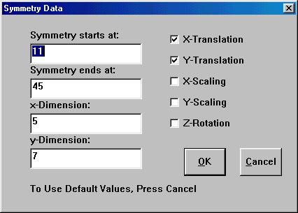
Select: "Data/Symmetry" to specify:
where symmetry ends
the x-dimension of the symmetry
the y-dimension of the symmetry
y-translation symmetry
x-scaling symmetry
y-scaling symmetry
z- rotation symmetry
Position 012 3456 789 10Click: 'Data/Symmetry' to open a dialogue box and specify:
Vector 100 0011 011 0
check
Symmetry starts at 3Symmetry ends at 10
x-dimension is 8
y-dimension is -1
x-dimension = Symmetry end - Symmetry start + 1 , orNote that this problem is for illustration of setting up the symmetry only. ABM 2.6 will not run for 11 neurons. You must have at least 30 neurons.
8 = 10 - 3 + 1.
Example The '5 by 7' Character Recognition Problem (See Chapter 2) has x- and y-translation symmetry. Let a pattern be:
01000 00000 0
00100
01100
00100
00100
00100
00100
01110
The class-neurons take bits from 0 to 10 and the pattern-neurons takes bits from 11 to 45. x-dimension is 5 and the y-dimension is 7. Click: 'Data/Symmetry' to open a dialogue box and to specify:
x-dimension * y-dimension = Symmetry end - Symmetry start + 1,
or 5 * 7 = 45 - 11 + 1.
When you specify the translation symmetry, the numbers
must satisfy the following conditions:
1-D: x-dimension = Symmetry end - Symmetry start + 1;2-D: x-dimension * y-dimension
= Symmetry end - Symmetry start + 1.
When there are errors in the specification, an error
message will be printed.
A symmetry is defined by five check boxes:
Setting Meaning
--------- -------------
00000 No symmetry
10000 x-translation
01000 y-translation
11000 x- and y-translation
00100 x-scaling and x-translation
10100 x-scaling and x-translation
01100 Not supported
11100 Not supported
00010 y-scaling and y-translation
10010 Not supported
01010 y-scaling and y-translation
11010 Not supported
00110 x- and y-scaling , x- and y-
translation
10110 x- and y-scaling , x- and y-
translation
01110 x- and y-scaling , x- and y-
translation
11110 x- and y-scaling , x- and y-
translation
00001 z-rotation, x- and y-translation
10001 z-rotation, x- and y-translation
01001 z-rotation, x- and y-translation
11001 z-rotation, x- and y-translation
00101 z-rotation, x- and y-scaling,
x- and y-translation
10101 z-rotation, x- and y-scaling,
x- and y-translation
01101 not supported
11101 not supported
00011 z-rotation, x- and y-scaling,
x- and y-translation
10011 not supported
01011 z-rotation, x- and y-scaling,
x- and y-translation
11011 not supported
00111 z-rotation, x- and y-scaling,
x- and y-translation
10111 z-rotation, x- and y-scaling,
x- and y-translation
01111 z-rotation, x- and y-scaling,
x- and y-translation
11111 z-rotation, x- and y-scaling,
x- and y-translation
Basically, ABM supports:
2D:
All neural computation starts with training. Training mean ABM learns the patterns from the training file.
After the training comes the recognition/testing. Recognition means ABM classifies the patterns in the recognition/testing files.
There are two commands:
Run/Classification -------- the Hopfield Model;
Run/Distribution --------- the Boltzmann Machine.
The output of the computation goes to the output file.
After clicking a command, the output file will be opened automatically.
The default output file name is "example1c.txt". You can change the output file name by clicking: "Data/Link", or its button on the toolbar, then type in your new data file name (See Figure 2).
The command, "Run/Distribution" (See Figure 5), presents you with a distribution, which is all possible classifications and how valuable the ABM thinks each prediction is via a confidence number. This number is similar to the number in an Internet Search Engine: the higher that number, the more confidence the ABM has in that distribution.
The command, "Run/Classification"(See Figure 5), presents you with a classification, and a confidence number. This number is similar to the number in an Internet Search Engine: the higher that number, the more confidence the ABM has in that classification.
Each of the above commands has two phases:
Click commands "Run/Classification" or "Run/Distribution", you can expect three possibilities for each testing pattern:
Incorrect classification: this is usually the case when: the Boltzmann Machine assigns a predominate probability to more than one configuration; or the relative probability is "small". It is hard to define "small" here because it depends on the problem, but for a given problem, an experienced user will know what is "small".
No classification: this is usually the case when
the Boltzmann Machine can find little correlation in the test pattern,
based on the current training. In such a case, "No classification " is
printed in the output data file.
If you are not sure of the correctness of the training and testing files, click: "Data/Test" to test the two files. If the formats of the files are not right (for example, the neuron numbers are inconsistent among the files), then the "Data/Test" command will tell you.
There are situations where
"Run/ Local Minimum (5)"
"Example/Double Shifter/Complete Patterns"
"Example/Triple Shifter/Complete Patterns"
"Example/Quad Shifter/Complete Patterns"
This command is used to fix the pattern: when a classification and part of the pattern are given, the network fixes the remaining part of the pattern.
This commands starts with a random configuration, and follows the network trajectory until it reaches the local minimum. The local minimum configuration is printed in the output file.
This option can fall into a local minimum and miss the global minimum. This option can not escape from a wrong local minimum. To escape from the wrong local minimum, we offer the next command, where you can start from many different points.
The two main commands,
Run/Distribution --------- the Boltzmann Machine.
The difference between command "Run/Local Minimum (1)" and command "Run/Local Minimum (5)" is the second command repeats the first command 5 times, i.e. this commands starts from 5 different random configurations. This provides a chance to avoid falling into wrong local minimum.
3.7 1-Neuron-1-Class Classifications
There is no restriction on how to represent a class using class neurons. The most common method to represent a class is to use one neuron for each class. Among class neurons, one of the neurons is '1'; all others are '0':
010 ... 00
001 ... 00
...
000 ... 10
000 ... 01
We call the above representation as "1 neuron for 1 class"
or 1N1C representation. If you do choose 1N1C representations, we have
two more commands:
Run/1N1C Classification -------- similar to Run/Classification;
Run/1N1C Distribution --------- similar to Run/Distribution.
The reason to offer these two commands is that they
are faster than "Run/Classification" and "Run/Distribution" commands, especially
for large problems.
If your problem is reasonably large, meaning:
3.8
Training, Retraining and Testing
Command Run/Classification is made up of two commands:
Common errors are: